


Many programs perform some computations more than once. For instance, a computational geometry application may need to solve multiple quadratic equations. How can we write the code below only once and simply “call it” whenever we need to solve a quadratic equation?
In the early days of computers, programs were called “routines”; therefore, reusable code fragments were naturally called “subroutines”, and later “subprograms”.
Subroutines in assembly language. Subroutines can be implemented in any language that has a “computed jump” instruction. For example, here is the outline of a subroutine that solves quadratic equations, written in an assembly language:
    ; Solve quadratic equation AX^2 + BX + C = 0
    ; Input: A in r1, B in r2, C in r3, return address in r4
    ; Output: solutions in r1 and r2
    quadratic:
            mul r5, r2, r2     ; compute solutions
            ...
            jmp r4             ; return to caller
In addition to the three parameters A, B and C, this subroutine takes a fourth parameter, which is the code address where the subroutine should jump to when it has finished. Each invocation of the subroutine sets this return address before jumping to the first instruction in the subroutine:
            mov r4, L100       ; set return address
            jmp quadratic      ; invoke subroutine
    L100:   ...                ; execution resumes here
Most instruction set architectures provide a call instruction that jumps to a given code address while storing the address of the next instruction in a register or on a stack. A single call instruction is sufficient to invoke a subroutine:
            call quadratic, r4   ; first invocation
            ...                  ; execution resumes here
            ...
            call quadratic, r4   ; second invocation
            ...                  ; execution resumes here
Nested subroutines, i.e. subroutines that invoke other subroutines, can be handled by storing the different return addresses in different registers r4, r5, etc., or by saving return addresses in memory, typically on a call stack.
Subroutines in Fortran I. Fortran I has computed jumps (the GOTO DEST command, where DEST is a variable) and the ability to set a variable to the value of a label (the ASSIGN LBL TO DEST command). This is enough to write subroutines in the same way as in assembly language, using variables to pass parameters and return addresses. For example:
Here is an invocation of this subroutine:
The simple subroutines described above are inconvenient for code reuse: the subroutines and the main program share all the variables, requiring great care to use different variable names in different subroutines. Fortran II in 1958, quickly followed by Algol in 1960, introduced better linguistic support for code reuse: procedures and functions. This support can be found in almost all programming languages today.
Subroutines and functions in Fortran II. Three types of subprograms with explicit parameters are supported in Fortran II: subroutines, simple functions, and general functions.
Subroutines correspond to what we now call procedures: commands that take parameters and can be called from multiple locations. For example, here is the quadratic equation solver in Fortran II:
And here is an invocation of this procedure:
The CALL command performs not only the transfer of control to the subroutine and back to the point after the call, but also the passing of parameters. Arguments that are variables or arrays are passed by reference. Thus, assignments to variables X1 and X2 in QUADRATIC are actually assignments to variables Y1 and Y2 in the caller. Other arguments are passed by value. Thus, variables A, B and C in QUADRATIC are initialized to 1.0, -2.0, and 5.0.
All variables are local to a subprogram or to the main program, unless they are declared COMMON. In the example above, the assignment to D in QUADRATIC has no effect on a variable D in the caller, since they are two different variables.
Simple functions in Fortran II are just expressions with parameters. For example, a function that linearly interpolates between two values A and B can be defined as
and used in expressions just like built-in functions SIN, COS, etc:
General functions, on the other hand, consist of one or more commands, like subroutines. To return a value to its caller, a function sets the variable whose name is the name of the function. For example, here is a function that computes and returns the average of an array of numbers:
Notice the assignment to AVRG on line 10: this is what defines the value returned by this function.
General functions are called within expressions, just like simple functions:
Procedures in Algol 60 are similar to the subroutines and general functions of Fortran II. Roughly speaking, a procedure is a block statement with parameters; it can optionally have a return value, making it usable as a function. Unlike Fortran II, however, Algol 60 passes parameters either by value or by name, depending on how parameters are declared. In addition, procedures can be recursive, nested within other procedures, and passed as arguments to other procedures.
Here is the quadratic equation solver as an Algol procedure:
The two parameters x1 and x2 are not declared value, and are therefore passed by name. Thus, assignments to x1 and x2 in quadratic affect the arguments provided by the caller, while assignments to a, b and c would have no effects outside of quadratic.
Here is a naive computation of an integral, as a function taking a function as a parameter:
Here is an example using integral that also demonstrates nested procedures:
Note that the inner procedure interpolate has access to the variables a, b of the enclosing procedure test.
Argument passing in Algol 60 is specified by the famous copy rule, which is given in the Report on the Algorithmic Language ALGOL 60 (Backus et al., 1960) as follows:
Any formal parameter not quoted in the value list is replaced, throughout the procedure body, by the corresponding actual parameter […] Possible conflicts between identifiers inserted through this process and other identifiers already present within the procedure body will be avoided by suitable systematic changes of the formal or local identifiers involved […] Finally the procedure body, modified as above, is inserted in place of the procedure [call] statement and executed.
This description is reminiscent of call by name in the lambda-calculus and related functional languages (see section 5.4), and of hygienic macro expansion in languages like Scheme. However, unlike lambda-calculus, Algol is an imperative language; combined with the copy rule, this leads to surprising behavior! Consider the following summation function:
This function is quite versatile and can be used
sum(i, 1, m, A[i])
sum(i, 1, n, i * i)
sum(i, 1, m, sum(j, 1, m, A[i,j]))
In the three examples, the copy rule replaces the loop index k with i and the argument ak with an expression that depends on i. Thus, the loop performs the expected summation. (This trick is known as “Jensen’s device”.)
The copy rule can also have unwanted effects that are hard to guess by reading the code. Consider the following procedure:
This procedure does not always exchange its arguments! For example,
swap(A[i], A[j]) works as expected, but
swap(i, A[i]) is, according to the copy rule, equivalent to
The assignment to i interferes with the subsequent assignment to A[i].
Because of these subtleties of the copy rule, and because it is difficult to implement correctly and efficiently, later languages in the Algol family such as Algol 68, Pascal, Ada, C and C++ abandoned call by name and used combinations of call by value and call by reference.
Terminology. In the rest of this chapter, we use “function” as a generic term for subprograms, subroutines, procedures, and functions. Subroutines and procedures can be thought of as functions that return no value, like functions of type void in C-like languages.
Design dimensions. Most programming languages support functions, with varying levels of expressiveness and usability. The following design dimensions can be identified:
These design choices are closely related to the implementation techniques used to represent runtime environments during execution. Runtime environments assign values to the variables that are in scope at a given point in the program. In compiled code, environments are materialized using various types of storage: processor registers, fixed memory locations, locations in a call stack, locations in a garbage-collected or explicitly-managed heap, etc. Depending on the strategy used to implement environments, some of the features of functions listed above may or may not be supported.
Statically allocated environments. This is the strategy used by the first Fortran compilers. Environments are represented by global, statically allocated memory locations: one location per COMMON variable; one location per variable and parameter of a function; and one location per function, to hold the return address in the caller of that function. Consider the program on the left:
DIMENSION A(10)

SUBROUTINE F(A, N)
  ... I ... J...

SUBROUTINE G(X, Y)
  COMMON A
  ... A ... I ... J ...
The representation of the environment is shown on the right. Note that the global variable A and the parameter A of subroutine F are placed in different memory locations, since they represent different program variables; the same is true for the local variables I and J of F and G.
This implementation technique is remarkably simple: all the memory used to represent the environment is allocated statically, at link time; no dynamic allocation takes place during program execution. Its main limitation is that it does not support recursion and other forms of reentrancy. For example, if function F above were recursive, there would be multiple bindings of local variables A, N, I, J active at the same time, and multiple return addresses in callers of F to record; this requires dynamic memory allocation of variable bindings and return addresses, typically on a stack.
Environments as stack frames. This approach uses a stack of activation records, also called stack frames. Each function call pushes a new frame onto the stack. This frame contains the values of the parameters, local variables, and return address for the called function. The frame is popped off the stack when the function returns. Global variables remain allocated statically.
Consider the Algol recursive procedures on the left and the stack on the right:
procedure g(x, y)
  integer x, y; value x, y;
begin
  integer i, j;
  ...
end;
procedure f(n)
  integer n; value n;
begin
  integer i;
  if n = 0 then f(1)
           else g(...)
end
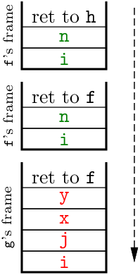
The stack grows downwards. The first call of f with argument 0, from another procedure h, say, pushes a frame with a return address into h and bindings for the variables n and i of f. Procedure f then calls itself recursively, pushing a second frame with a return address into f and bindings for n and i. The second activation of f, with argument 1, calls g, pushing the third frame shown at the bottom of the stack, with a return address in f and bindings for the variables and parameters of g.
This stack-based implementation of environments is almost universally used in programming language implementations today. It naturally supports recursion. If nested functions are forbidden, like in C but unlike in Algol, it also supports functions as first-class values: the value of a function is just a code pointer, pointing to the entry point of the function’s code. Since all free variables1 of a non-nested procedure are global variables, which are statically allocated, there is no need to pass dynamically-allocated parts of the environment to the function when it is called.
Stack frames for nested functions. In the case of nested functions, as in Algol, a function must have access to the local variables of its enclosing functions. This can be achieved by chaining the stack frames following the nesting of functions: the stack frame for a function activation contains a pointer, called an access link, to the stack frame for the latest activation of the immediately enclosing function. By traversing this chain of stack frames, the value of any variable visible to a function can be retrieved.
Consider the following variant of the previous example, where procedure g is now nested inside procedure f:
procedure f(n)
  integer n; value n;
begin
  integer i;
  procedure g(x, y)
    integer x, y; value x, y;
  begin
    integer j;
    ...
  end;
  if n = 0 then f(1)
           else g(...)
end
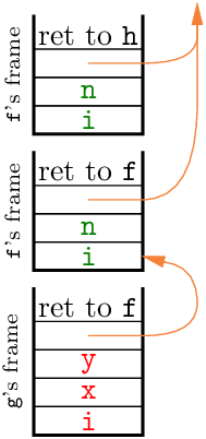
Note the access link (orange arrow) from the frame of g to the frame for the most recent call of f, the procedure that encloses g. This link allows g to access the variables i and n declared in f. Likewise, both frames for f contain an access link pointing to the most recent frame for the procedure that encloses f, if any, or a null pointer if there is no enclosing procedure. Note also that access links do not link stack frames in the order in which they appear on the call stack: the caller of a function is generally not the immediately enclosing function, as shown in the example above for the recursive call to f.
In this approach, function values cannot be represented as mere code pointers, since free variables of functions can now be local variables of other functions, whose values are to be found in dynamically-allocated stack frames. Therefore, function values must be represented as closures: pairs of a pointer to the function code and a pointer to the chain of stack frames corresponding to the enclosing functions. However, these function closures have short lifetimes: the chain of stack frames is invalidated as soon as one of the enclosing functions returns. For this reason, Algol and Pascal allow functions to be passed as arguments to other functions, but not to be returned as function results, nor to be stored in data structures.
Heap-allocated closures and objects. To remove these restrictions on functions, and to be able to use them as first-class values, we need to allocate function closures and parts of runtime environments in a memory heap that does not follow a stack discipline. This way, closures are not invalidated when functions return; they remain usable throughout program execution, if the heap uses automatic memory management (garbage collection), or until deallocated by the program, if manual memory management is used.
Naively, we could heap-allocate all activation records for all function calls. However, this can be expensive. A better alternative is to heap-allocate only those parts of the runtime environment that are actually needed by function closures, namely the values of the free variables of the functions. This is the approach taken by most functional languages today: a function closure is a heap-allocated record with the first field containing a pointer to the code of the function, and the remaining fields containing the values of the free variables of the function. A stack of activation records is still used to store return addresses and variable bindings that are not captured in a function closure.
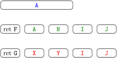
For example, consider the OCaml function fun x -> a * x + b, where a and b are free variables, bound outside the function. When this function is evaluated in a context where a is 2 and b is 5, the following function closure is constructed on the heap:

The code of the function is shown here in C syntax. It is a closed function that takes as its first argument the closure itself, from which it can retrieve the values of the free variables a and b. Applying this closure c to argument 8, for example, amounts to calling the function c->code and giving it c as an additional argument, as in c->code(c, 8).
This kind of self-application semantics is also used by object-oriented programming languages. The runtime representation of an object (an instance of a class) is similar to that of a function closure: a record containing the values of the instance variables of the class, plus a pointer to a “v-table” mapping method names to code pointers. The code that implements a method gets a pointer to the object as an extra argument, giving the method access to the instance variables. From this perspective, a function closure can be thought of as an object with a single apply method, and an object can be thought of as a function closure with multiple entry points (one per method).
Simple function calls. In Fortran II, the flow of control around a function call is simple: when the function returns, execution always continues with the command that syntactically follows the call. In other words, the invocation CALL proc(e1, …, en) is a base command, just like an assignment x = e, except that the call is not guaranteed to terminate. In addition, since code labels are local to functions, a function cannot jump to another function using goto.
Multiple return points. In Fortran 77, a subroutine can have other return points besides the point after the CALL. These alternate return points are labels passed as additional arguments.
For example, here is a solver for quadratic equations that returns to an alternate point if there are no real solutions:
And here is an example of use:
Each * (asterisk) character in the parameter list represents an alternate return point. It corresponds to a label (here, *99) in the argument list of CALL. The RETURN 1 statement means “branch to the first alternate return point”, while a plain RETURN statement means “branch to the default return point”.
Non-local goto. In Algol 60 and its descendants, a goto L command can jump out of one or more enclosing blocks as long as the goto is in the scope of the definition of label L. This works even if the goto is in a different procedure than the definition of L, as long as the scoping constraint is respected.
Consider the following Algol program:
Any call to fatal_error anywhere in the program will print an error message and jump to the terminate label, which is at the very end of the program, causing the program to terminate immediately.
Algol also supports passing labels as arguments to procedures. This can be used to implement procedures with multiple return points, in the style of Fortran 77. For example, here is a quadratic equation solver with error handling:
Pascal does not support labels as function arguments, but the same effect can be achieved by passing a procedure whose body is a goto to the desired label.
This use of non-local goto is more powerful than Fortran 77’s multiple return points: the label err passed to quadratic is not necessarily defined in the caller of quadratic, but can be defined in any enclosing function. Therefore, goto err does not necessarily return to the caller, and can jump anywhere in the call stack.
Exceptions. This idiom of “jumping out of a function” to signal an error can also be achieved using exceptions in languages such as C++, Java, Python, or OCaml. Exceptions and exception handling are discussed in details in chapter 9. In short, exceptions are supported by two language constructs. The first, written throw in Java, raises an exception: this stops the current computation and jumps to a handler for the exception. The second construct, written try s1 catch (ex) s2, intercepts exceptions ex raised during the execution of command s1 and executes command s2.
Here is an example of error reporting and error handling with exceptions in Java:
When an exception is raised by a throw statement, the call stack is dynamically searched for a caller function that has a try statement that can handle the exception. Some try statements can be skipped (if they cannot handle the exception), but their finally clauses are always executed.
The main difference between exceptions and non-local goto is that the handler of an exception, i.e. the target of a throw statement, is determined entirely dynamically, while the target of a goto statement is determined by the goto statement itself. This makes exceptions more flexible and easier to use, but it also results in less predictable control flows and greater risk of forgetting to handle an exception. Section 9.4 discusses these problems and possible workarounds in more detail.
Chapter 9 of Scott and Aldrich (2025) gives a nice overview of subroutines, parameter passing modes, structured exceptions, and their stack-based implementations. Section 9.3 of Pratt and Zelkowitz (2000) also discusses various semantics for parameter passing and their implementation. Chapter 7 of Aho et al. (2006) gives more details on the implementation techniques for runtime environments and the different types of functions they support.
The use of closures to implement first-class functions with lexical binding originates in Landin (1964) and was popularized by the Scheme language (Sussman and Steele, 1975). Chapter 15 of Appel (1998) describes the compilation of a functional language using closures. This can be compared with the compilation of an object-oriented language as described in chapter 14 of the same book.