


Thus far, we have taken for granted that source code must explicitly describe the sequencing of computations in a program, and that programming languages must provide control structures to express this sequencing. However, this assumption is questioned by declarative languages, which leave the sequencing of computations mostly implicit in the source code and rely on the compiler to determine the correct order of computations. In other words, declarative languages emphasize the what (what is to be computed?) rather than the how (how to break the computation in elementary steps? in which order to perform these steps?).
An example of the declarative approach is database query languages such as SQL: the query describes which records to pull from the database; how to search the database is left to the database management system to decide. Other declarative programming paradigms include logic programming (Prolog, Datalog), pure functional programming (Haskell, Agda), and dataflow programming (Simulink, Lustre). Hardware description languages such as Verilog and VHDL are also declarative in nature.
Declarative languages were introduced in the 1970s with the goal of simplifying programming and “liberating it from the von Neumann style”, as Backus (1978) put it. In the 1980s, the focus shifted to parallel computation: it was hoped that declarative languages would be easier to execute in parallel than standard imperative languages, precisely because the former give the compiler more flexibility in scheduling computations. Since the 1990s, declarative languages have been recognized for their safety and their proximity to formal verification.
Can declarative languages do without control structures? Do they “liberate” programmers from the burden of expressing control in their programs? This chapter attempts to answer these questions in the context of pure functional programming, by examining three little languages with increasing expressiveness: XL, a spreadsheet language; APP, an applicative language with functions distinct from values; and FUN, a functional language with functions as values.
Expressions with sharing. Consider the following language of arithmetic expressions and equations, nicknamed “XL”:
| Expressions: e | ::= | 0 ∣ 1.2 ∣ 3.1415 ∣ … | constants | |||
| ∣ | x ∣ y ∣ z ∣ … | variables | ||||
| ∣ | op(e1, …, en) | operations | ||||
| Programs: p | ::= | { x1 = e1; …; xn = en } | sets of equations |
Arithmetic expressions such as x + 1 and y × z are built from constants and variables using operations such as +, −, ×, /, etc. Programs are sets of equations between variables and expressions.
The use of variables that are bound to expressions by equations captures a notion of sharing of computations. For instance, the two programs
|
compute the same results (in a sense to be made precise later), but p1 can evaluate 2 × 3 only once and share the result 6 in the evaluation of x + x, while p2 evaluates 2 × 3 three times.
Spreadsheets such as the one shown in figure 5.1 can be viewed as visual displays of sets of equations:
|
The variables are the spreadsheet cells B2, C6, etc. Cells containing manually-entered values represent trivial equations variable = constant. Cells containing formulas give rise to nontrivial equations variable = formula.
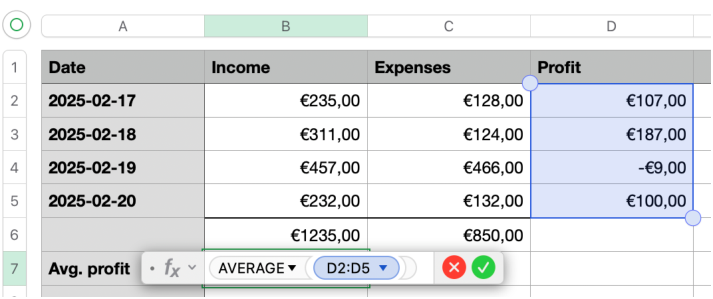
Figure 5.1: A simple spreadsheet.
The acyclicity condition. We want XL programs to be easy to evaluate. This means avoiding equations that are difficult to solve, such as x = x3 − 2x2 + 2. We go much further and rule out all equations x = e where e depends on x, either directly or indirectly through other equations, as in the following examples:
|
In other words, the equations must not contain a dependency cycle. This acyclicity condition holds if and only if the program can be written not just as a set of equations, but as an ordered list of equations
| x1 = e1; …; xn = en |
where the only variables that can occur in ei are the variables xj for j < i.
Figure 5.2: The spreadsheet as a combinatorial circuit.
Figure 5.3: The spreadsheet as a dataflow graph. (Σ stands for the SUM operator and A for the AVERAGE operator.)
Circuits and dataflow graphs. Figures 5.2 and 5.3 show two alternative presentations of the spreadsheet of figure 5.1. The first is a circuit, with variables (cells) represented by wires and operators by gates. The acyclicity condition corresponds to the absence of loops in the circuit. In other words, this must be a combinatorial circuit.
The other alternative presentation is a dataflow graph: a directed acyclic graph (DAG) with constants and operators as nodes, and edges representing the flow of data (from a node to an operator that requires its value). The acyclicity condition corresponds to the absence of cycles in the graph.
Program evaluation. Evaluating an XL program { x1 = e1; …; xn = en } consists in determining the numerical value vi of each variable xi. These are the values that are displayed in the cells of the corresponding spreadsheet.
Without committing to a specific evaluation algorithm, we can describe all possible evaluations as successive reductions of the program. Each reduction rewrites the program as another, simpler program. The evaluation process is complete when the program has been rewritten as a set of trivial equations { x1 = v1; …; xn = vn }, from which the value vi of the variable xi is readily apparent. Here are the two reduction rules that can be used:
|
These rules can be applied anywhere in the right-hand side of an equation. Rule (unfold) is analogous to the “copy rule” of Algol (section 3.2): it states that a variable x can always be replaced by the expression e associated with x by an equation.
Rule (prim) describes the evaluation of an operator op applied to values v1, …, vn, which is replaced with its result value v. We write op* for the interpretation of the operator op. For example, if we take +* to be the floating-point addition of 32-bit floating-point numbers, we have 123000 + 0.005 → 123000.008.
Here is an example of a sequence of reductions:
|
In a given program, reduction rules can often be applied to different subexpressions, resulting in multiple reduction sequences for this program:
|
However, all reduction sequences terminate with the same fully-evaluated program. This is a consequence of the following confluence property of rules (prim) and (unfold):
Evaluation strategies. Although all reduction sequences produce the same result, some sequences are more costly than others — sometimes exponentially so. Consider the following program:
| {x0 = 1; x1 = x0 + x0; … ; xn = xn−1 + xn−1} |
Using a “call by name” evaluation strategy, we replace each xi with its definition before performing any arithmetic evaluations. This results in an intermediate state
| {x0 = 1; x1 = 1+1; x2 = (1+1)+(1+1); x3 = ((1+1)+(1+1))+((1+1)+(1+1)); … } |
of size 𝒪(2n), which then needs 𝒪(2n) reductions by rule (prim) before evaluation is complete.
Using a “call by value” evaluation strategy, we reduce the expression that defines xi to a value vi before replacing xi with vi. This results in the following intermediate states:
|
We only need 2n reductions to evaluate the program.
For the XL language in this section, the “call by value” strategy is optimal. This strategy is captured by the following restriction of rule (unfold):
|
If the program is represented as an ordered list that respect dependencies, this strategy can be implemented by the following evaluation function, which returns the final, fully-evaluated program:
|
We write eval(e) for the value of a closed expression e (one that does not contain any variables), obtained in linear time by repeated applications of rule (prim).
Adding function definitions. We now extend the XL language of section 5.2 with the ability to define functions F with one or more parameters x1, …, xn, and to call these functions within expressions.
| Expressions: e | ::= | true ∣ false ∣ 0 ∣ 1.2 ∣ … | constants | |||
| ∣ | x ∣ y ∣ z ∣ … | variables | ||||
| ∣ | if e1 then e2 else e3 | conditional | ||||
| ∣ | op(e1, …, en) | built-in operations | ||||
| ∣ | F(e1, …, en) | function application | ||||
| Definitions: def | ::= | x = e | variable definition | |||
| ∣ | F(x1, …, xn) = e | function definition | ||||
| Programs: p | ::= | def ; … ; def |
To make examples more interesting, we also added Boolean values and a conditional expression if e1 then e2 else e3, which returns the value of e2 or the value of e3 depending on the truth value of e1.
To facilitate evaluation, we write programs as ordered lists of definitions, with the constraint that a definition can only mention function parameters and variables defined by previous definitions, but can mention functions defined later. This criterion ensures the absence of dependency cycles that do not go through a function application, while still allowing for recursive functions.
For example, here is a function F that computes the Fibonacci sequence, and a definition x for the 20th number in this sequence.
|
Here is an alternate definition of the Fibonacci sequence, closer to an iterative algorithm:
|
Notice that the APP language supports general recursion. Computations may not terminate (e.g. G(−1, 0, 1) in the example above). Indeed, APP contains Kleene’s partial recursive functions and is therefore Turing-complete.
Control structures in APP. On the one hand, the APP language is undoubtedly declarative in nature. In particular, there is no explicit sequencing of computations, only data dependencies that force certain operators to be evaluated before others. For instance, in the expression (1 + 2) × 3, the addition must be performed before the multiplication.
On the other hand, APP definitely supports two essential control structures: conditionals and loops. Conditionals are supported by the expression if e1 then e2 else e3, which is similar to an if…then…else statement in an imperative language (i.e. the then or the else branch is executed depending on the value of the Boolean expression e1).
Loops are supported by tail-recursive functions, i.e. functions where the recursive calls are performed as the final action of the function. For example, the following tail-recursive function
| G(n, a, b) = if n = 0 then a else G(n−1, b, a+b) |
is similar to the following imperative loop
Many types of loops can be expressed as tail-recursive functions, including for loops, while loops, do…while loop, with single-level break and continue.
Mutually-recursive functions can express even more complex forms of loops, which would require goto jumps in imperative languages. For example,
|
is similar to the following unstructured imperative code, whose control-flow graph is irreducible:
More generally, any flowchart can be expressed as a set of mutually-recursive functions, as observed by McCarthy (1960, section 6).
Evaluation strategy. For conditionals and loops to work as expected, we must constrain the evaluation strategy beyond just “any order of evaluation that satisfies the data dependencies”. As a trivial example, if…then…else conditional expressions must not evaluate both the then and else branches before selecting one of their values; otherwise, a loop such as
| G(n, a, b) = if n = 0 then a else G(n−1, b, a+b) |
would diverge (not terminate) for any value of n, evaluating infinitely many recursive calls to G with n−1, n−2, …
Clearly, the conditional expression if e1 then e2 else e3 must not be “strict” in its three arguments: e1 should first be evaluated to a Boolean b before starting the evaluation of e2 (if b is true) or of e3 (if b is false). It is less obvious how to evaluate function applications: should they be “strict” in their arguments or not? We will return to this question in the next section, where it will be discussed in the context of the richer FUN language.
Constants: c ::= true ∣ false ∣ 0 ∣ 1.2 ∣ … Expressions: e ::= c constants ∣ x ∣ y ∣ z ∣ … variables ∣ λ x . e function abstraction ∣ e1 e2 function application ∣ if e1 then e2 else e3 conditional expression
Figure 5.4: Abstract syntax for the toy functional language FUN.
Function abstractions in expressions. Another way to extend the XL language of section 5.2 with user-defined functions is to add function abstractions λ x . e and function applications e1 e2 to the language of expressions e. There is no need to distinguish between function names and variable names: a variable x can represent any value, including functions. Unlike in APP, functions can be nested and refer to free variables of enclosing functions.
The syntax for this extension, called FUN, is summarized in figure 5.4. The expression λ x . e represents the function that maps the argument x to the result e. A function that takes n arguments x1, …, xn can be defined as λ x1 . λ x2 … λ xn . e. Applying such a function f to n arguments e1, …, en is written as n−1 applications to a single argument
| f e1 e2 ⋯ en = (⋯ ((f e1) e2) ⋯) en |
A multi-argument function like f is called a curried function, in honor of logician H. B. Curry. If we add operators (+, −, etc) as constants, we can also view arithmetic operations such as x + y as curried function applications such as ((+) x) y.
The syntax in figure 5.4 does not include definitions and appears to lack support for recursion. As will be explained later, these features can be expressed in terms of the core constructs of the FUN language. Nevertheless, the following examples will use recursive definitions.
Higher-order functions. In the FUN language, functions are first-class values: they can be used anywhere a numerical or Boolean value can be used, including as arguments to other functions.
Functions that take functions as arguments are called higher-order functions. They provide new ways to compose and reuse sub-programs. For instance, function composition f ∘ g is definable as a higher-order function, as is function exponentiation f ∘ ⋯ ∘ f (n times):
|
Here is a generic loop that iterates the function step, starting with x, until the predicate stop becomes true:
| Iter = λ stop . λ step . λ x . if stop x then x else Iter stop step (step x) |
Higher-order functions can express generic traversals of data structures such as lists. For instance, Map applies a function to each element of a list and Fold reduces a list using a two-argument function.
|
Encoding definitions. The examples above show FUN programs as lists of definitions x1 = e1 ; … ; xn = en. However, it is not necessary to include these definitions in the abstract syntax of FUN, since they can be encoded as expressions.
A non-recursive definition x = e ; … becomes a let binding let x = e in …, which is just a function application:
| let x = e in e′ ≜ (λ x . e′) e |
A simply-recursive definition f = e becomes a let rec binding let rec f = e in e′, which is itself defined using a fixed-point combinator Y:
| let rec f = e in e′ ≜ let f = Y (λ f . e) in e′ |
For example, the Exp function shown above is defined as follows:
| Exp = Y (λ E . λ f . λ n . if n = 0 then λ x . x else Compose f (E f (n−1))) |
The fixed-point combinator Y can be defined as
| Y ≜ λ f . (λ x . f (λ v . x x v)) (λ x . f (λ v . x x v)) |
Finally, mutually-recursive definitions can be expressed in terms of simply-recursive definitions. Here, we show the encoding for two mutually recursive definitions, f = e1; g = e2.
|
Reduction rules. As in section 5.2, we view the evaluation of a FUN expression as a sequence of reductions. Each reduction rewrites the expression in order to perform one step of computation. Here are the reduction rules we need:
|
The rule (λ x . e) e′ → e [x := e′] is known as the beta reduction of the lambda calculus. It captures the essence of function application: the formal parameter x is replaced with the effective argument e′ in the body e of the function.
In rule (prim) and elsewhere, we write v for a value, which can be either a constant or a function abstraction.
| Values: v | ::= | c ∣ λ x . e |
Here are some examples of reduction sequences. We take Δ = λ x . x x and Ω = Δ Δ.
|
As shown by examples (ii) and (iv), some terms have infinite reduction sequences, which means divergence (non-termination). As shown by examples (iii) and (iv), a given term can have both finite and infinite reduction sequences, depending on which subterm we choose to reduce at each step.
These examples demonstrate that the reduction rules alone do not uniquely determine the meaning of a FUN program. Therefore, we must specify a reduction strategy that constrains where and when the reduction rules can be applied to evaluate an expression.
Evaluation strategies. All functional programming languages use only weak reductions: they prohibit reductions within function abstractions (“under a lambda”) and in the then and else branches of a conditional; instead, they wait until the function is applied or the Boolean condition of the if-then-else is known before reducing further. As mentioned at the end of section 5.3, non-weak reductions, also called strong reductions, are problematic in combination with general recursion, since they often lead to non-termination.
Restricting ourselves to weak reductions still leaves us with a choice of strategy for function applications:
Call by name avoids divergence as much as possible, but may duplicate computations. For example, writing Fib for the recursive Fibonacci function and Ω for an expression that diverges, we have:
|
Call by value avoids repeated evaluations, such as the one of Fib 20 in the last example above, but it can diverge unnecessarily:
|
Call by need attempts to offer the best of both worlds: it avoids divergence just like call by name, and it avoids repeated evaluations just like call by value. However, the sharing of evaluations comes with conceptual difficulties and implementation costs.
|
The two occurrences of Fib 20 come from the substitution of the same variable x. Therefore, their evaluations are shared: when the evaluation of one occurrence terminates with value 6765, the other occurrence is known to have value 6765 as well.
Haskell uses call by need as the default strategy for function application. Most other functional programming languages (Lisp, Scheme, SML, OCaml, etc.) use call by value, as do all modern imperative and object-oriented languages. Call by name played an important role in Algol 60 (see section 3.2); today, it is only used for compile-time macro expansion and template expansion.
Encoding evaluation strategies. Even if our language is call by value, we can implement call by name semantics by passing arguments e as thunks: functions λ z . e where z is a fresh variable not used in e. As long as we stick to weak reduction, e will not be reduced in the thunk λ z . e until it is applied to a dummy argument.
This idea gives rise to a systematic program transformation 𝒩(e) that ensures that all function applications in e use call by name:
|
We obtain call by need instead of call by name if we use memoized thunks (lazy e in OCaml) instead of plain thunks λ z . e.
Implementing call by value in a call by name or call by need language is more challenging. One approach is to use a CPS (continuation-passing style) transformation, as explained in section 6.5. Haskell provides primitive operations that force the evaluation of a function argument, such as the seq operator and the $! strict application operator.
How can we formalize and define an evaluation strategy with mathematical precision? The approach we follow throughout this book is to define evaluation in terms of reductions under restricted contexts.
Contexts. A context is an expression with a hole, written as [ ]. For example, (1 + [ ]) × 3 is a context.
If C is a context and e an expression, C[e] denotes the expression obtained by replacing the hole [ ] in C with e. For example, if C = (1 + [ ]) × 3 and e = 2/5, then C[e] = (1 + 2/5) × 3.
Reductions under contexts. Using contexts, we can more precisely explain what it means to apply a reduction rule “anywhere in an expression”, as we have done so far. We define whole-program reductions p → p′ as head reductions e →ε e′ under reduction contexts C, as follows.
|
In more words, reducing a program p proceeds as follows:
For example, if 1 + 2 →ε 3 is a head reduction, then 4 × (1 + 2) → 4 × 3, using the context C = 4 × [ ].
If we allow any context to be used as the reduction context C, whole-program reduction can take place anywhere in the program. However, we can constrain where reductions can take place by restricting which contexts C can be used as reduction contexts, thus specifying a reduction strategy.
Weak reduction is described by the following grammar of reduction contexts:
| C ::= [ ] ∣ C e ∣ e C ∣ if C then e2 else e3 |
This grammar does not allow λ x . C nor if e1 then C else e2 nor if e1 then e2 else C as reduction contexts. Therefore, reductions cannot take place in a function body (“under a lambda”) or in the then or else branches of a conditional.
The head reduction rules for FUN are the four rules described in section 5.4:
|
Call by value is obtained by replacing the β head reduction with
| (λ x . e) v →ε e [x := v] (βv) |
This prevents the reduction of an application until its argument has been evaluated to a value v. This is the essence of call by value.
Optionally, we may want to specify an evaluation order for applications e1 e2. Left-to-right evaluation, where we evaluate the function part e1 before the argument part e2, is enforced by the following grammar of reduction contexts:
| C ::= [ ] ∣ C e ∣ v C ∣ if C then e2 else e3 |
We allow v C as a context but not e C: the argument part of the application can only be reduced if the function part has already been evaluated.
Symmetrically, right-to-left evaluation is enforced by taking
| C ::= [ ] ∣ C v ∣ e C ∣ if C then e2 else e3 |
Call by name uses the unrestricted β rule
| (λ x . e) e′ →ε e [x := e′] (β) |
This makes it possible to pass arguments e′ unevaluated to functions. Additionally, call by name ensures that arguments cannot be evaluated before being passed by restricting evaluation contexts as follows:
| C ::= [ ] ∣ C e ∣ if C then e2 else e3 |
There is no context that allows reducing e′ in (λ x . e) e′; the only reduction that can take place here is the (β) rule.
Call by need is difficult to describe in terms of reduction rules. The problem lies in the β rule (λ x . e) e′ →ε e [x := e′]: all occurrences of the parameter x in the function body e must share the same argument e′, to ensure that when one occurrence of x is replaced by the value v of e′, all other occurrences are replaced as well. One solution is to represent expressions by directed acyclic graphs (DAGs) instead of terms, and view reduction rules as graph rewriting rules instead of term rewriting rules. This approach uses the same reduction rules and the same reduction contexts as for call by name.
Ariola et al. (1995) develop another approach to call by need, using variable bindings in terms to represent sharing. The language of expressions is enriched with explicit let bindings:
| Expressions: e | ::= | … ∣ let x = e1 in e2 |
Function application let-binds the function argument to the function parameter, instead of substituting one for the other:
|
It is only when the argument e′ has been reduced to a value v that this value v can be substituted for x:
|
Other rules are provided to lift let-bindings to the top of the expression:
|
Reduction contexts are those of call by name, extended with two cases for let bindings:
|
The context let x = C in C′[x] captures the essence of call by need: we can reduce the expression bound to a variable x only if the value of this variable is needed for the rest of the program to make progress, i.e. only if the rest of the program can be written as C′[x] for some evaluation context C′. Since contexts are recursive, these two types of let contexts can capture arbitrarily long chains of dependencies, as in let x = C in let y = C′[x] in C″[y].
Chapter 1 of Structure and Interpretation of Computer Programs, the textbook by Abelson and Sussman (1996), is a classic introduction to declarative programming from a functional perspective. The textbook by Van Roy and Haridi (2004) discusses declarative programming in greater details, particularly from the perspectives of logic and relational programming.
Part 1 of Pierce (2002) explains untyped functional languages (such as our FUN toy language) and their formal semantics. The use of reduction contexts was introduced by Wright and Felleisen (1994) and is explained again and compared with other styles of operational semantics in chapter 5 of Harper (2016).
Part 2 of Peyton Jones (1987) describes the implementation of lazy evaluation using graph reduction.

