


Nowadays, “structured programming” refers to the uncontroversial practice of writing programs using high-level control structures (conditionals, loops, …) rather than low-level goto jumps. In the period 1965–1975, however, structured programming was the subject of much debate, both as a movement toward a new perspective on software, and as a controversy about how to write good programs.
The structured programming movement pushed for a radical change in the way we look at software. In the early 1960’s, the standard view of a program was flowcharts as the high-level description, and assembly code or other low-level programming as the materialization of that description.
Structured programming promotes a view of a program as a constructed, structured source text, written in a high-level language. This source text should be understandable on its own, without the need to refer to flowcharts or other external documentation, and should support reasoning about the program, informally at first, mathematically later (using program logics).
The manifesto for this movement is the book Structured programming by Dahl et al. (1972). The three essays in this book introduce high-level programming concepts that have had a profound influence on modern software engineering: formal methods, program refinement, data structures, type algebras, objects and classes, and coroutines. Whether programs should be written with or without goto is an irrelevant detail from this book’s perspective.
The structured control controversy focused on much narrower issues than the structured programming movement. It was a dispute between two styles of programming: on the one hand, programs with many goto statements obtained by naive transcription of a flowchart; on the other, programs using exclusively or almost exclusively control structures (conditionals, loops, …), written directly without the help of a flowchart. This dispute became known by the slogan Go to statement considered harmful, from the title of a famous paper by Dijkstra (1968).
Early sightings. Knuth (1974) lists early sightings of structural programming in the computer literature. For example, in 1966, Dewey Val Schorre mentions the use of textual, indentation-sensitive outlines instead of flowcharts to document assembly code:
Since the summer of 1960, I have been writing programs in outline form, using conventions of indentation to indicate the flow of control. I have never found it necessary to take exception to these conventions by using go statements.I used to keep these outlines as original documentation of a program, instead of using flow charts …Then I would code the program in assembly language from the outlines. Everyone liked these outlines better than the flow charts.
In 1963, Peter Naur criticizes goto statements and the use of flowcharts:
If you look carefully you will find that surprisingly often a go to statement which looks back really is a concealed for statement. And you will be pleased to find how the clarity of the algorithm improves when you insert the for clause where it belongs.If the purpose [of a programming course] is to teach Algol programming, the use of flow diagrams will do more harm than good, in my opinion.
Sparking the controversy. It is Dijkstra’s short communication Go to statement considered harmful (Dijkstra, 1968) that sparked the controversy about structured control. He sent it as a letter to the editors of Communications of the ACM, without a title; the editors added the now-famous title. In typical Dijkstra style, this text begins with a bang:
For a number of years I have been familiar with the observation that the quality of programmers is a decreasing function of the density of go to statements in the programs they produce. More recently I discovered why the use of the go to statement has such disastrous effects, and I became convinced that the go to statement should be abolished from all “higher level” programming languages (i.e. everything except, perhaps, plain machine code). At that time I did not attach too much importance to this discovery; I now submit my considerations for publication because in very recent discussions in which the subject turned up, I have been urged to do so.
The paper then describes Dijkstra’s “killer argument” for why goto should be abolished. It has to do with the difficulty of “knowing where we are” in the execution of a program, and of describing and reasoning about the path taken from the beginning of the program to the current point in the execution.
For programs consisting of a sequence of basic operations, the current program point is sufficient to describe the execution path. For if-then-else conditionals, we also need to know the Boolean values of the previous conditionals. If the program point is inside one or several structured loops, we also need to know how many times these loops have been executed. Consider:
The execution path is completely described by a small set of coordinates, as Dijkstra puts it: the iteration counts for the two loops, the Boolean value of the x == 0 test for each iteration, and the current program point.
However, if the program uses arbitrary go to statements, “it becomes terribly hard to find a meaningful set of coordinates in which to describe the process progress”, as Dijkstra writes. Consider:
The goto statement creates a loop that partially overlaps the two conditionals, making it difficult to describe the possible execution paths. This kind of programs with convoluted execution paths is commonly called “spaghetti code”, for visually obvious reasons.
Programming without goto statements was the subject of many studies in the early 1970’s: first, to assess whether purely structured programming was really the best way to express program structure, as opposed to disciplined use of goto; then, to design methods for eliminating goto statements in existing programs, either on a case-by-case basis or systematically by program transformation.
Knuth’s survey, Structured Programming with go to Statements (Knuth, 1974), discusses the effects of eliminating goto on well-chosen examples, noting that it can reduce code clarity or decrease performance, especially if it causes duplication of code fragments or addition of Boolean flags.
Here is an example, adapted from Knuth: insertion into a hash table using linear probing. The table is represented by two arrays: A[N] containing the keys and B[N] containing the associated values.
This C code is very concise, yet fairly self-documenting, owing to the two labels notfound and found. It does, however, contain two goto statements.
We can rewrite it using a structured while loop with no early exits and no goto, as follows:
However, the test A[i] == 0 is duplicated and may cause runtime overhead, unless the compiler optimizes aggressively.
Another attempt uses a while loop with a (structured) early exit via a break statement:
What ends up being duplicated here is the storing of the data B[i] = d, which occurs in both the “not found” and the “found” branches. This does not significantly affect readability nor performance, however.
Another, more modern example where goto statements are hard to avoid in C code is error handling with resource freeing. This is a common idiom in system code written in C: when an error occurs, use goto to jump to the code that frees the resources acquired so far, so that this resource-freeing code can be shared between all errors and with the no-error case.
Consider a function that opens a file and allocates temporary memory:
The epilogue of the function, which frees the resources buf and fd before returning the error/success code, is written only once; the error cases jump to the label err3, err2 or err1, depending on which resources were allocated before the error.
This code can easily be rewritten to not use goto, but at the cost of duplicating the freeing of resources, and at the risk of not freeing them consistently:
As in the previous example, loops with early exits allow us to share the error handling code while avoiding goto statements. The loops are degenerate (do ... while(0) executes its body exactly once); they play the role of blocks with early exits.
These examples suggest that goto statements can be replaced with structured constructs, but this may require extra run-time tests or code duplication. Is this always the case? The remainder of this chapter provides answers to this question.
A technical question that played a central role in the structured programming controversy was the “goto elimination problem”: is it always possible to transform an unstructured program (written using goto and if…goto) into an equivalent structured program (using Algol-style blocks, conditionals, and loops)?
It turns out that this problem has a simple solution if we allow the structured program to have more variables than the original:
This result is easy to prove by explicitly constructing the structured program from the original program. Consider an unstructured program consisting of sequential computations s1, s2, …, sn (typically, sequences of assignments and procedure calls), with control expressed by labels 1, 2, …, n, unconditional jumps goto ℓ, and conditional jumps if b then goto ℓ, where b is a Boolean expression.
      1: s1
         if b1 then goto 3
      2: s2
         goto 4
      3: s3
      4: s4
         if b4 then goto 1
First, we reformat the program as a set of basic blocks: sequential computations systematically terminated by an unconditional jump goto ℓ or a two-way conditional jump if b then goto ℓ1 else goto ℓ2. This materializes fall-through behavior as explicit jumps to the immediately following label. We also add a special label “0” to denote the end of the program. In the example above, this results in:
      1: s1
         if b1 then goto 3 else goto 2
      2: s2
         goto 4
      3: s3
         goto 4
      4: s4
         if b4 then goto 1 else goto 0
Next, we introduce a new integer variable pc (the program counter) that ranges over the labels 0, 1, …, n and denotes the next basic block to be executed. The goto statements become assignments to pc. Basic blocks become the cases of a multi-way conditional statement on the value of pc.
    case pc of
        1: s1
           if b1 then pc := 3 else pc := 2
        2: s2
           pc := 4
        3: s3
           pc := 4
        4: s4
           if b4 then pc := 1 else pc := 0
    end case
Finally, we add a while loop that repeats the case statement until pc is zero, at which point the program terminates.
    pc := 1;
    while pc != 0 do
      case pc of
        1: s1
           if b1 then pc := 3 else pc := 2
        2: s2
           pc := 4
        3: s3
           pc := 4
        4: s4
           if b4 then pc := 1 else pc := 0
      end case
    end while
The construction above can be thought of as the iteration of a transition function. The transition function is implemented by the case multi-way conditional; it executes the basic block specified by the pc variable, updating pc and the other variables accordingly. The iteration is implemented by the while loop, which executes transitions until pc is zero.
Several variants of this construction are known: the integer variable pc can be replaced by multiple Boolean variables; the multi-way case conditional can be replaced by a cascade of if-then-else conditionals.
A folklore result. Theorem 1 is often attributed to C. Böhm and G. Jacopini. However, their 1964 article Flow diagrams, Turing machines and languages with only two formation rules (Böhm and Jacopini, 1966) shows a weaker result (any flowchart can be rewritten into a structured program with multiple while loops and Boolean auxiliary variables), using a more complex proof based on local graph rewriting.
Theorem 1 and the simple proof outlined above appear in 1967 in a letter by D. C. Cooper to the Comm. ACM editors (Cooper, 1967). As Harel (1980) describes, the theorem and its simple proof have been mentioned as “the mathematical justification of structured programming” in dozens, probably hundreds of papers and textbooks since 1967, rarely attributed to Cooper, often attributed to Böhm and Jacopini, often not attributed at all.
Harel traces the result back to S. C. Kleene’s 1936 proof that every partial recursive function is the minimization of a primitive recursive function. Here, the original flowchart is the partial recursive function, the case-based transition function is the primitive recursive function, and the while loop is Kleene’s minimization operator.
As a generalization of the goto elimination problem, Kosaraju (1974) introduced the notion of reduction of control structures between two languages.
Consider two programming languages ℒ1 and ℒ2 that support the same base commands (assignments, procedure calls, …) but differ in their control structure (for example, one has structured conditionals and loops and the other only has goto and if-goto).
Example 1: do-while loops, with the loop test at the end of each iteration, are not Kosaraju-reducible to while loops, with the loop test at the beginning of each iteration. Indeed, in order to eliminate
we must either duplicate s, as in
or use an additional Boolean variable, as in
In contrast, do-while loops are reducible to while loops with early exits (break):
The two conditions set by Kosaraju hold: no duplication of the base command s and no additional variables.
Example 2: cycle-free flowcharts are not reducible to if-then-else structured conditionals. Nested conditionals naturally describe trees of base commands; however, they are unable to capture the sharing of base commands present in acyclic graphs without resorting to code duplication or additional Boolean variables. Consider the following flowchart, for instance:

Using structured conditionals, we must either duplicate the command s2:
or add a Boolean variable recording whether we need to perform s2 later:
However, if our target language also has blocks with early exits block … break … endblock, we have a proper Kosaraju reduction:
As the examples above suggest, early loop exits (break statements) and multi-level exits (break N, where N is the number of nested loops to exit) make a big difference. Kosaraju (1974) proves that the language of loops with early exits is not reducible to a language with plain loops, and that a language with exits at level N+1 is not reducible to a language with exits at level N or less.
Control-flow graphs (CFGs) are a formalization of flowcharts. CFGs are often used as an intermediate representation (IR) for programs in compilers: they can represent both structured and unstructured control, and support many program transformations, static analyses and optimizations.
A CFG is a directed graph. A node of a CFG is a basic block: a sequence of basic commands (assignments, function calls, etc.) ending in a control transfer such as an unconditional branch, a conditional branch, or a function return. The edges of a CFG represent all such possible transfers. A node has one outgoing edge if it ends in an unconditional branch, two if it ends in an if-then-else conditional, N if it ends in a N-way conditional, and none if it ends in a function return.
For example, here is a small structured program and its corresponding CFG:

The notion of dominance is useful for analyzing the structure of a CFG. We say that a node A of a CFG dominates a node B if A is necessarily executed before B: every path from the entry node to B goes through A. Consider this CFG:

Each node dominates itself. The entry node A dominates all nodes. Node D dominates E, since there is no other way to reach E than going through D. In contrast, B does not dominate D, since the path ACD avoids B, and likewise C does not dominate D. Similarly, neither D nor E dominates A, since the trivial path A avoids D and E.
Dominance leads to a classification of CFG edges. We say that an edge U → V is a back edge if its destination V dominates its source U; otherwise, it is a forward edge. In the example above, the edge E → A is a back edge, and all other edges are forward edges.
Back edges naturally correspond to loops in the CFG: if we have an edge U → V, and if V dominates U, we also have a path V →* U, and therefore a cycle U → V →* U. However, not all loops involve back edges. In the example above, there is a loop between nodes B and C, but neither dominates the other.
Reducible CFGs are those CFGs where all loops involve back edges. More precisely, a CFG is reducible if its forward edges form an acyclic graph.
In the example above, the CFG is not reducible, since after erasing the back-edge E → A we still have a cycle between nodes B and C. However, the CFG below, which has no edge from C to B, is reducible: no cycle remains after deleting the back-edge E → A.

There are several other, equivalent definitions of reducibility. For example, a CFG is reducible if and only if it can be shrunk to a single node and no edges by repeatedly applying the transformations T1 and T2 below:
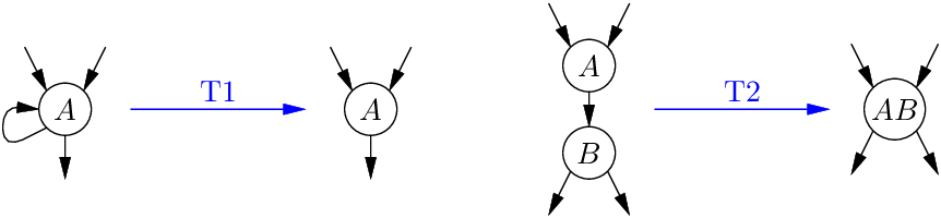
T1 removes self-loops, and T2 collapses a node B with its only predecessor A.
One aspect of reducible CFGs that makes them easier to analyze and optimize than general CFGs is that each loop is a natural loop and has a single loop header. Formally, a loop L is a strongly-connected set of nodes. It is a natural loop if there is a node H ∈ L (the loop header) that dominates every node in L, and such that every node in L has a path to H that stays within L.
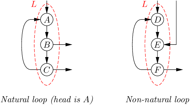
In the example above, ABC is a natural loop with header A. While it has two exit points at B and at C, it can only be entered through A. In contrast, DEF is not a natural loop because it can be entered in two different places: at the top D or in the middle E. As a result, D does not dominate E, and there is no loop header.
Structured control is closely related to the reducibility of CFGs. In one direction, all the control structures we have seen so far produce a reducible CFG once compiled. This includes conditionals (if-then-else, multi-way switch), loops (with tests at beginning, at end, or in the middle), and early exits (return, break, continue). In fact, all of these constructs produce natural loops with unique loop headers. To get a irreducible CFG, we would need a loop that can be entered in two different places: either a structured loop with a goto jumping inside the loop, or an unstructured loop made entirely with goto statements. If our source language does not support general goto, non-reducible CFGs cannot arise.
In the other direction, we have the following theorem, first proved and published by Peterson et al. (1973):
The proof by Peterson et al. is constructive: it outlines an algorithm that, given a reducible CFG, constructs an equivalent structured program. However, this algorithm consists in three passes and is quite complex. Ramsey (2022) recently published a simpler, one-pass algorithm that proceeds by induction on the dominator tree for the given CFG.
The dominator tree has the same nodes as the CFG. The children of node A are the nodes B that have A as immediate dominator, meaning: A ≠ B, A dominates B, and there are no dominators “in between” A and B (if A dominates X and X dominates B, then X = A or X = B).

For example, the CFG on the left above has the dominator tree shown on the right. Node A has four children: B and D, which are immediate successors of A in the CFG, but also E and F, which are not immediate successors but can be reached in two different ways from A.
Ramsey’s algorithm proceeds by recursion on the dominator tree. For each node, a structured command is produced, incorporating the structured commands produced for each children of the node. Let us start with the root A. It is a loop header, hence a loop is generated:
A has two children B and D in the dominator tree that are immediate successors in the CFG. Hence, a conditional statement over A is generated, with B and D as “then” and “else” branches. However, A has two other children E and F in the dominator tree, which we need to put just after blocks, so that they can be jumped to with break statements. This results in the following shape:
Note that E must go in the inner block and F in the outer block, since E flows to F. Ramsey’s algorithm uses a reverse postorder numbering of the CFG to determine this nesting of blocks.
Now we recurse on the four sub-dominator trees, inserting the resulting commands in the placeholders marked B, D, E and F above. We obtain:
All what remains to be done is to fill the dots with commands that implement the control transfers specified by the CFG. These commands can be nothing if control just falls through, or break N to terminate N enclosing blocks or loops, or continue N to restart the N-th enclosing loop. Here, C needs to continue with F, two enclosing blocks away, so a break 2 command is needed. D’s “then” branch continues with E, one block away, so we use break 1. D’s “else” branch continues with A, the loop header, so we use continue 1. Finally, we obtain the following structured program:
The reader is referred to (Ramsey, 2022) for the complete Haskell code of the algorithm and a proof sketch of its correctness.
Knuth’s survey (Knuth, 1974) gives a nice historical summary of the debate about structured programming in the late 1960’s and early 1970’s. It is also interesting as a very balanced perspective from an expert 1970’s programmer on the appropriate use of goto statements and on better language support for alternative, structured programming idioms.
Control-flow graphs and their use as intermediate representations are discussed in many compiler textbooks. Cooper and Torczon (2004) gives a good overview of control-flow graphs (section 5.2) and of dominance and dominator trees, including their relevance for the static single assignment (SSA) intermediate representation (sections 9.2 and 9.3). Aho et al. (2006), section 9.6, discusses loops, dominators and reducibility in more details.
The translation of reducible CFGs to structured programs is beautifully explained by Ramsey (2022), including a Haskell reference implementation and an extensive discussion of earlier work. Ramshaw (1988) reports on the elimination of goto statements in a significant code base (the Pascal sources of TEX), while retaining the structure of the original code as much as possible. Similar issues arise when decompiling from machine code to high-level structured languages (Brumley et al., 2013, Yakdan et al., 2015).